Numerical Solution of Heat Transfer Partial Derivatives Equation

Abstract

In this project, the numerical solution of the two-dimensional unsteady heat transfer equation has been discussed using the explicit method, ADI and ADE. TDMA is used for the equations formed in the ADI method and finally the results of these three methods have been compared. All codes are written in c++ language.

1. Introduction

In this project, the transient two-dimensional heat transfer problem is analyzed using numerical methods. Heat transfer is a significant issue in computational fluid dynamics (CFD), with numerous applications in mechanical engineering and various industries. The project aims to solve the heat transfer equation numerically by employing three different methods: the explicit method, the ADI (implicit) method, and the ADE (hybrid) method. Each method has its own characteristics and advantages. For instance, the explicit method offers simplicity and fast calculations, but it requires small time steps to maintain stability. In contrast, the ADI method is unconditionally stable, allowing larger time steps, though it is more complex to implement.

A non-uniform mesh is used in the problem to better capture the steep temperature gradients near the boundaries. Finally, the results from all three methods are compared, evaluating their effectiveness in simulating the heat transfer process.

2. Methodology & Solution

In this project, the geometry consists of a two-dimensional square plate where heat transfer occurs steadily through conduction. The plate is defined with fixed temperature boundary conditions on all four walls:

• Right wall: 25 Kelvin
• Left wall: 200 Kelvin
• Top wall: 0 Kelvin
• Bottom wall: Zero gradient (Neumann boundary)

Heat conduction occurs throughout the plate, and the goal is to find the temperature distribution in this geometry. When thermal properties (such as thermal conductivity) are constant, the heat transfer equation is simpler to solve. However, when properties vary, the equation becomes more complex, requiring greater precision in the solution.

Solution Methods:

Explicit Method: In this method, the temperature at each point in the next time step is calculated using only the temperatures of neighboring points from the current time step. This method is simple and does not require solving a system of equations. However, due to the need for small time steps to ensure stability, it results in longer computation times.

ADI Method (Implicit): This method solves the problem in two stages. In the first stage, the equations are solved implicitly in the x-direction and explicitly in the y-direction. In the second stage, the roles are reversed, solving implicitly in the y-direction and explicitly in the x-direction. This method is unconditionally stable, allowing for larger time steps, though it is more complex to implement.

ADE Method (Hybrid): In this explicit method, instead of using values from the previous time step, current time step values are used for the calculations. This method has a shorter execution time compared to ADI and is suitable for specific boundary conditions (Dirichlet type).

In all these methods, the goal is to compute and compare the temperature distribution in the plate over different time intervals.

3. Flow Simulation and Validation Results

The important equation used is the Transient Two-Dimensional Heat Transfer Equation:

Equation (1):

\[ \frac{\partial T}{\partial t} = \alpha \left( \frac{\partial^2 T}{\partial x^2} + \frac{\partial^2 T}{\partial y^2} \right) + Q \]

This equation serves as the foundation for calculating the temperature distribution in the plate.

Stability Condition for the Explicit Method:

\[ \text{Stability condition} = \Delta t \leq \frac{\Delta x^2}{2 \alpha} \]

This condition ensures the stability of the explicit method in time steps.

Temperature-Dependent Thermal Conductivity Relation:

\[ k = aT + b \]

This relation is used to calculate variations in thermal conductivity based on temperature.

In short, the results are as follows:

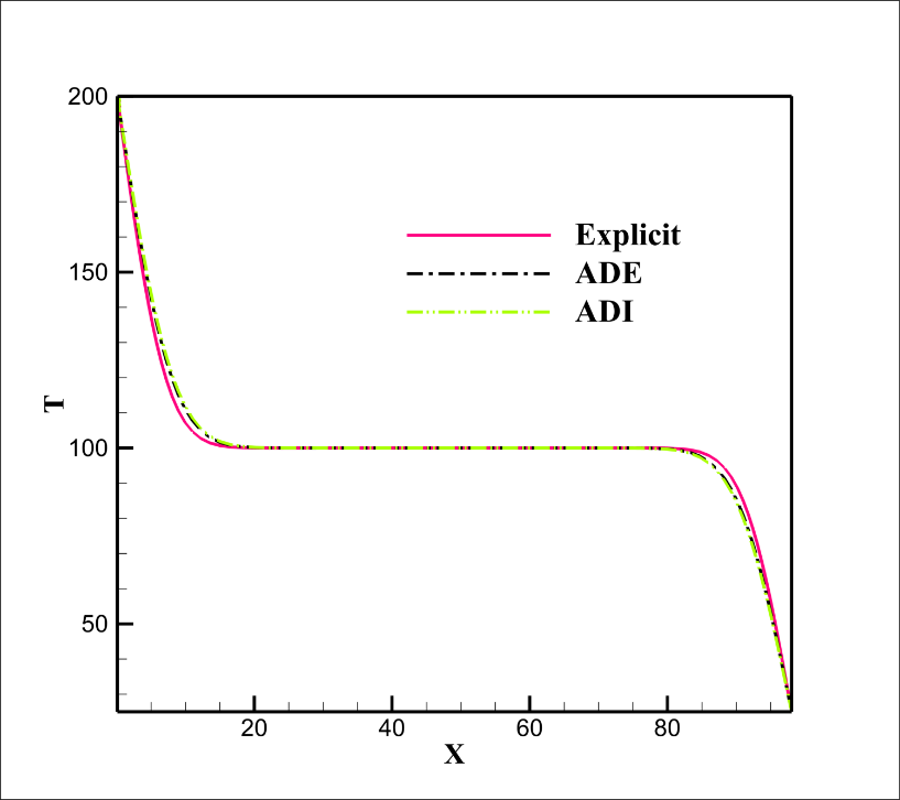
As it is clear from the contours and the graph, the results of the three methods are consistent for a time of 20 seconds. And from now on, due to the same results, only the results of the ADE method, which has a shorter execution time than the ADI method, are reported.

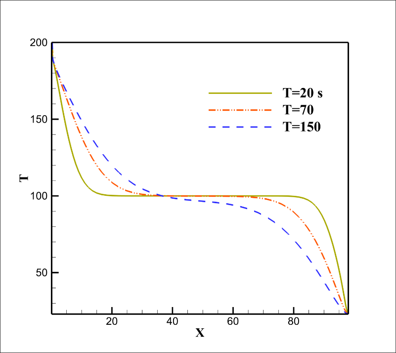
Also, the diagram of the main diameter and the center of the hole in the y direction can be seen in Figures 2 and 3, and the thermal penetration can be understood by increasing the program execution time.